Budget Planning with Excel: Cell Format

Tip Number 2: Make ordinary numbers appear as dates and currency.

I use a worksheet for each month of the year. The lefthand column of the sheet gives the date. You don't have to type 1-Jan, 2-Jan, 3-Jan, etc for the whole month. Excel can interpret a positive integer as a date. Here's how it works.

1 = January 1, 1900
2 = January 2, 1900
. . .
40,179 = January 1, 2010

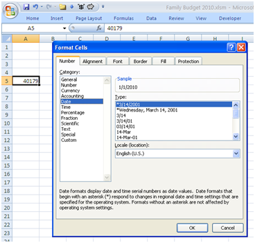
So try this: Put "40179" in cell A5. Right-click A5 and choose "Format cells." Select "Date" from the Category box and choose the Type on the right. You'll see a preview in the Sample window.

Now your 40179 is transformed into a date.

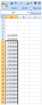
To populate the rest of the dates for the month, create a formula in A6: "=A5+1". After you hit Enter, A6 should show 1/2/2010. You can copy A6, select the next 30 rows or so, and select Paste. You now have a month of dates.

You can redo this for every month (February 1, 2010 = 40,210), or I suppose you could do the whole year in one sheet.

The format for most cells in the sheet (everything east of column A and south of row 4) will be Currency. I prefer the format that shows negative numbers in red with parentheses. When the cells are set up like this, Excel will automatically interpret an entry like "4.1" as $4.10 and -38.5 as ($38.50). High visual contrast and a minimum number of keystrokes. That's what I like.