Budget Planning with Excel: Freezing Panes

Here's Tip Number 1: Learn how to freeze panes properly. This is a feature of Excel that never works the way I think it should, but it is possible to freeze the leftmost column(s) and topmost row(s) so that they're always visible when you scroll elsewhere in the document.

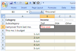
In Excel 2007, the Freeze Panes command is on the View tab. Pre-2007, it's under Window.

The trick is to select the cell that will be in the upper left-hand corner of the lower right-hand quadrant before choosing "Freeze Panes." Got that?

If you select the cell highlighted as "This one!" in the picture above, you'll freeze the top two rows and the leftmost column so they're always visible.

At the risk of belaboring the point, it may help to think of this command as cutting the sheet into four quadrants (the "panes"). Excel will make a cut along the top of the selected cell and along its left side.

If you mess up, there doesn't seem to be a way to adjust where the "cuts" lie. You just have to unfreeze the panes and try again.

(HT: Tech Xpress)